Disease Detection - Experiments in ML Challenges

Problem Statement

The prediction problem I aim to solve is classifying select diseases based on an input of patient experienced symptoms. The beneficiaries of a problem like this being solved is any person who feels they are becoming ill and wants to obtain a quick diagnosis based on their symptoms. This type of model could either be a chat bot deployed by a hospital to talk with patients and give them an estimated diagnosis based off their symptoms, or an easily accessible website that does the same task previously described but for any user (not limited to only hospital patients).

Data Set

The sources for my data comes from Kaggle from two different pages, the first being the Disease Symptom Prediction data set and the second being the Predict Disease Symptom data set. The original authors for both data sets are Pranay Patil and Pratik Rathod, who collected the data from different sources on the web. Along with the data set being used, a data set was created where they ranked each symptom on a scale from [0,10] based on the severity over a two day period (also included on both Kaggle pages).

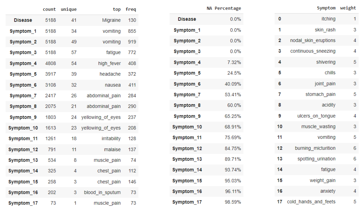
• Data Set (Left) - this data information is a combination of the two data sets, which were combined to only keep classes that were shared between the two sets (small minority classes that were mostly duplicates were dropped). The class label is denoted by the Disease feature, which contains 41 unique diseases across 5,188 observations. Since all features are filled with symptoms that are in the format of strings, no summary statistics could be provided. However, each symptom feature does tell us how many total unique symptoms were experienced by all observations and what the most frequent symptom is. One note is that the symptom features do not correspond to any sort of importance or ordering based on which feature they appear in (i.e. values in Symptom_1 are equally important as values in Symptom_15).

• Missing Values (Middle) - the missing values are a bit different in this data set since there can be a total of 17 symptoms present for any given observation, but not all disease produce 17 symptoms. Due to this, missing values will not be encoded to preserve the missing information (all symptoms will be converted to binary indicators, 1 if present and 0 if not). As we can see the number of missing values increases as the number of symptoms increases, which is expected since not all diseases have a large amount of symptoms. There are a total of 3 features that have no missing values, so all diseases experience at least 3 symptoms but less than half of the observations have over 7 symptoms still.

• Severity Data (Right) - the severity data set contains all 139 symptoms found in the data set, with a corresponding weight that describes how severe the symptoms effect is on the body over a 2 two day period. This data will later be used for the challenge of creating/replacing features in the original data set.

Model Definitions

Since all symptoms are considered to be either present or not, I utilized tree-based classifiers since I believed they would create good test cases for the branches. For example if some branch tests for a specific symptom being present or not, then that branch could lead to good class separation if a large majority of diseases do not have that symptom and only a small number experience that symptom. This led to using a Decision Tree and Random Forest Classifier for the two models in the project. I wanted to use a Decision Tree as a comparison to the Random Forest in order to determine if a simple or more complex version of similar classifiers would perform equivalent, or if there was a large enough performance increase in using the Random Forest to quantify the more complex model. The largest weakness for both the Decision Tree and Random Forest Classifier are the extensive leaf nodes and the test cases used to separate the classes. This can lead to overfitting if the models try to perfectly separate the data, which will perform well on training data but not generalize well to new data (too specific in decision boundaries). This can be amplified in the Random Forest if all trees are performing this overfitting, and lead to even worse test set performance. The hyperparameters for each model are specified below:

• Dummy Classifier - this is the baseline estimator, with the strategy being set to “most frequent” and the random state as 42.
• Decision Tree - the default parameters were used for this classifier, which has a max depth that goes until each leaf node has perfect separation. It uses the gini criterion to measure the quality of the splits, and performs the splits based on the best separation. The random state is also set to be 42 so that the model’s results are reproducible.
• Random Forest - the default parameters were used for this classifier, with the number of estimators being set at 100 trees in the forest. It uses the gini criterion to measure the quality of the splits, and performs the splits based on the best separation. The random state is also set to be 42 so that the model’s results are reproducible.

Evaluation Setup

For evaluation of models across each challenge, I implemented 5-fold stratified cross-validation and evaluated based on the following metrics: accuracy, f1-score, precision, and recall. For all evaluation metrics, the parameter for average was set to “weighted” in order to account for the multi-class labels. This calculates the metric for each class label and then takes the weighted average between them as the final score. Although class labels are initially balanced, I utilized stratified CV in order to ensure a class would not disappear in the train/test splits in any fold. Accuracy and f1-score are the main metrics to focus on, with F1-score being slightly more important as we want to reduce the number of incorrectly classified diseases. Since cross-validation is being used, the metrics presented in the results section are the average across all folds during the training/evaluation process. Although class labels are balanced in the original data, in the duplicate removal methods I wanted to ensure that each class maintained it’s importance when dropping observations. For my baseline estimator, a dummy classifier was utilized in order to predict the majority class (performance is not expected to be high due to large number of classes present).

ML Challenges + Proposed Solutions

For each challenge and the three solutions within them, the dimensions of the resulting data sets are given in order to compare differences in size based on proposed solutions/methods. The data was formatted with each symptom being converted to a binary indicator and the original string symptoms being dropped (this resulted in 139 features, all containing either 1 or 0 for each observation).

1. Duplicates

While exploring the data, the classes were nearly balanced (120-130 observation for each) and led me to believe that there may be duplicates in the data set. After looking through the data, there seemed to be a large portion of the data being duplicated in order to balance each disease class. This leads to the question of how to handle duplicates so that there are not repeated observations in both the training and test sets, which will be solved with one of the following proposed solutions:

• Do Nothing (5,188x139) - the first option is to leave the duplicates in the data set and train/evaluate the model on all of the data. This method I would expect to result in nearly perfect accuracy, since duplicates will most likely occur in both the train and test set. This will lead to shared observations between the two sets, and due to this will cause the model the predict on observations it has already seen during training.
• Remove Duplicates (334x139) - the second option, and most likely to represent the true performance of the model, will be to remove the duplicates in the data set. There is a large portion of the data that is duplicated, and doing this will result in only 334 observations remaining in the new data set (which also needs to be split between train and test sets). This is a very small amount of data to use for the model and make any type of statements about, which led me to the final proposed solution.
• Randomly Removing Symptoms (1,177x139) - the final option is to create a new data set by randomly dropping one symptom that is present in each row in an attempt to increase the non-duplicated data set size from solution 2. This will be done across the entire data set, including duplicated and non-duplicated observations, and then filtered to only keep the non-duplicated observations. One note is that the classes are no longer approximately balanced, but partially reflects the non-duplicate class distribution and did not decrease overall performance. The function is reproducible and produces the same data set each time (drops same random symptom index each time).

2. Feature Selection

When formatting the data, each symptom was converted into a binary indicator to mark whether or not it was experienced in the corresponding observation. However, after doing this the data became very sparse since the majority of observations had less than 7 out of 17 symptoms. There were 682,383 values set as 0 (not present) and only 38,749 values set as 1 (symptom was present). Since tree based classifiers typically don’t work as well with sparse data, this lead to the challenge of exploring if reducing the number of features in the data set would improve model performance. The following solutions are proposed for this challenge:

• Use All Features (1,177x139) - the first solution is equivalent to “do nothing”, where all symptom binary indicators will be used as input to the model. I would expect this data set to maintain the best performance since it contains the most information from the three proposed solutions, but aiming to maintain similar performance with the other two proposed solutions will be the goal for this challenge.
• Use Top-N Features (1,177x50) - the second option will be to utilize only the top-n features as inputs to the model (selecting n by the most frequent symptoms in the data set). I’m a bit unsure how this will perform since the top features are highly shared among multiple disease classes, so they will not provide much information for separating them. Another option to look at is using the n least frequent symptoms, or a combination of the two.
• Principle Component Analysis (1,177x21) - the third option will be to utilize Principal Component Analysis in order to reduce the number of features in the data set but still maintain the maximum amount of information. I will aim to maintain at least 80% of the variance in the data set, conditional on the idea that the number of principal components is substantially lower than the original number of features. The cut-off for variance comes from previous statistics courses and PRINCIPAL COMPONENTS (PCA) from UCLA.

3. Symptom Severity}

Along with the original data, there is another data set which contains each symptom and its associated severity score [1,10] on the body over a 2 day period. I imagine this this information would be more meaningful than a binary indicator, as it can convey the weight associated with a symptom rather than it just being present in the observation. This brings up the challenge of how to use this data in order to enhance or replace the current features in the data set, and will be solved by one of the following proposed solutions:

• Original Features (1,177x139) - the first solution will be to do nothing and use the original features as inputs, ignoring symptom severity. This will be used as a comparison to the other two proposed solutions to evaluate changes in performance due to new features.
• Average Symptom Severity (1,177x1) - the second solution will be to take the average symptom severity (sum of all symptom severity’s divided by number of symptoms) and use this as a single input feature. I do not believe this will perform well, as having 41 classes and only a single input feature will most likely have matching inputs to multiple classes and lead to poor separation.
• Severity Ranking (1,177x18) - the third solution will be to create features for the severity rankings. This will convert severity ranges to new features, mapped as {“Low”: 1-3, “Moderate”: 4-6, “High”: 7-10} and converted to binary indicators for each. If an observation has a symptom that falls in one of these ranges, or multiples ranges, they will be set as 1 (otherwise 0). Another feature to consider adding will be the number of symptoms, which will contain the count for how many symptoms will be present (ranging from 1 to 17) and converted to binary indicators to stay consistent in formatting and data ranges.

Results

Duplicates

The first challenge found in this data set was determining how to handle the duplicate observations, which were compared across three different solutions. For handling the encoding of the features, each symptom is represented as a binary indicator. The results for the baseline and two classifiers are represented in the table below.

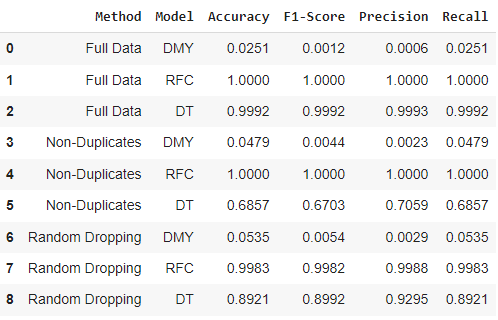
From this challenge, we can see that the two classifiers (RFC and DT) have slightly different performance on the same proposed solutions. As expected, the baseline (DMY) performance is very low for each solution due to the large number of class labels. For both solution 2 and 3, the Random Forest performs much better than the Decision Tree (as expected), and so when accounting for duplicates the more complex model seems to be more appropriate for this problem. As expected, solution 1 of leaving duplicates in the data set resulted in 100% for all evaluation metrics due to information being shared between the train/test splits. For solution 2 of removing all duplicates, the Random Forest had perfect classification while the Decision Tree seemed to struggle in the mid 60%’s for its evaluation. For solution 3 of randomly dropping symptoms from observations, again the Random Forest performed approximately 10% better on all evaluation metrics compared to the Decision Tree. It was surprising how much higher the Decision Tree performance from solution 2 to solution 3 was (approximately +30% for all metrics), and leads me to think that the very small data set (334 observations) from solution 2 was a factor in the poor performance. Based only on metrics the Random Forest with solution 2 performed the best, but I would prefer to use/deploy the solution 3 since it has more data ($\sim$3.5x) and greatly increased the Decision Tree performance.

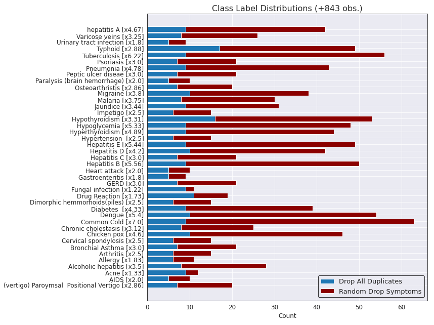
The figure below shows a breakdown of the difference on class distributions between solution 2 (using only non-duplicate observations) and solution 3 (randomly dropping a disease from each observation). The y label also contains the overall increase for solution 3 compared to solution 2 for each class label in the data set.

Feature Selection

The second challenge from in this data set was exploring different methods to reduce the number of features in the data set (currently 139 binary indicators). For the data set being used, this comes from the challenge 1 solution 3 of randomly dropping one symptom per observation and will be used from both this challenge and challenge 3 to be consistent. The results for the baseline and two classifiers are represented in the table below.

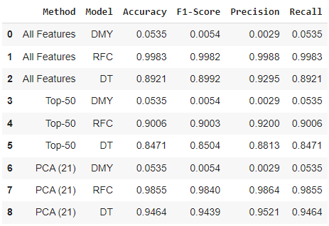
From this challenge, we can again see that the two classifiers (RFC and DT) have slightly different performance on the same proposed solutions. As expected, the baseline (DMY) performance is very low for each solution due to the large number of class labels (always predicting Common Cold as the disease - majority class from Figure 4). Solution 1 of using all features had the same performance as challenge 1 solution 3 from Figure 3, with the Random Forest performing around 10% better on all metrics. For solution 2, the 50 most frequent symptoms were used as binary indicators and performance slightly decreased due removing less frequent symptoms that help to separate disease classes. The performance was slightly higher than I expected for both models, but would not be a solution I would use moving forward in the project or in a real world application. For solution 3, 21 principal components were selected to maintain 80.24% of the variance in the original data. This method works surprisingly well, with the Random Forest maintaining it’s performance and the Decision Tree performance increasing by roughly 5% for all metrics compared to using all original features. Moving forward in a real world application, I would utilize the solution of PCA since it reduced the number of input features from 139 to 21 and either maintained or increased both models performances.

Symptom Severity

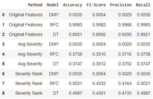
The third challenge from this data set was utilizing the symptom severity data set in order to create or replace features in the original data. For the data set being used, this comes from the challenge 1 solution 3 of randomly dropping one symptom per observation and the challenge 2 solution 1 of using all original features (can’t use PCA solution since it is not possible to replace features with symptom severity in principal component format). The results for the baseline and two classifiers are represented in the table below.

From this challenge, we can see that the two classifiers (RFC and DT) had very similar performance on both solution 2 and solution 3 (results from solution 1 still follow previous challenge 2 solution 1 of $\sim$10% difference between models). Again, the baseline (DMY) performance is very low for each solution due to the large number of class labels. For solution 2, both models performances were a large drop from using the original data (decreasing anywhere between 50-60% on all evaluation metrics). Interestingly, the Decision Tree performed better than the Random Forest by an extremely small margin (less than 0.1% on all metrics). For solution 3, both models performed almost identical on all metrics again with $\sim$13% increase over the solution 2 performance. A sample from the data set created is provided on the bottom of Figure 6, and is very interesting that the models still learned how to separate some classes despite only knowing the severity ranking and number of symptoms (no information on what the symptom actually is). Moving forward, solution 2 and 3 would not be something I would use in a real world application but was an informative experiment on different ways the data could be formatted and still learned from (and possibly could be used in combination with the original binary indicators or PCA to increase performance).

Final Solutions

From each challenge and proposed solutions above, the overall best method for each was found to be:

• Challenge 1: Randomly dropping one symptom per observation to reduce the number of duplicates (better performance on evaluation metrics compared to the non-duplicate data set and overall increased data size, with +843 observations).
• Challenge 2: Using PCA to reduce the number of features and maintain/increase model performance (similar/better performance on evaluation metrics compared to using all features and reduced computation for model, with only 21 features instead of 139).
• Challenge 3: Using all original features without symptom severity performed the best (performance greatly decreased when utilizing only severity for creating the features used in the training/evaluation).