
Throughout these projects, a variety of tools were utilized in order to perform analysis and provide insights based on the chosen data sets. From using a Compute Engine Instance to obtain and transfer data to a GS Bucket, to uploading Python scripts to run PySpark jobs using Dataproc, the following projects provide an general introduction to using the Google Cloud Platform tools. Specifically, the following discussed projects cover the following:
- Compute Engine Instances
- Google Storage Buckets
- Dataprep
- BigQuery
- Dataproc
Compute Engines, Dataprep, & BigQuery
Obtaining the Data (Compute Engine Instance)
The problem of increasingly large dataset sizes has led to local computing hardware becoming a limitation, which has the impact of increasingly expensive computing resources needing to be purchased in order to handle them. Cloud computing tools, such as Google Cloud, allow us to work with these large datasets online with limited local computing resources being needed. A good starting point to familiarize ourselves with this cloud computing pipeline would be to work with a large dataset, and perform similar tasks as to what we have seen with the smaller projects in the course. This project covers this pipeline from obtaining a large dataset, processing/cleaning it, and finally performing analysis on it; all through Google Cloud tools.
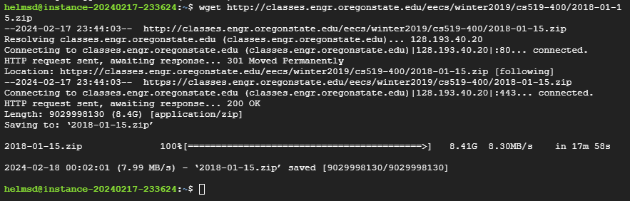
Data was obtained from a URL provided in the assignment instructions, specifically a zip file that contains 2,359 JSON files on a wide variety of information regarding flights. To obtain the data, a Compute Engine Instance was created on Google Cloud in order to use wget and download the zip file from the provided link. The below screenshot shows the success of this process:
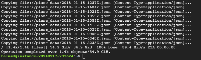
Once downloaded, then all JSON files were extracted using the unzip command. After all files were extracted, gcloud tools had to be initialized before we could begin transferring the data. Once initialized, all of the JSON files were then copied from the Compute Engine Instance into the Google Cloud Storage bucket (named cs512_flight_data). The below screenshot shows the success of this process:
Once all files had been uploaded to the GS bucket, they were then loaded into Dataprep. I did run into the issue of the JSON files showing, but when previewing the dataset it was empty. I read through the FAQ on the assignment page, updated the path to remove the extra forward slash, and was able to successfully preview the dataset.
Cleaning the Data (Dataprep)
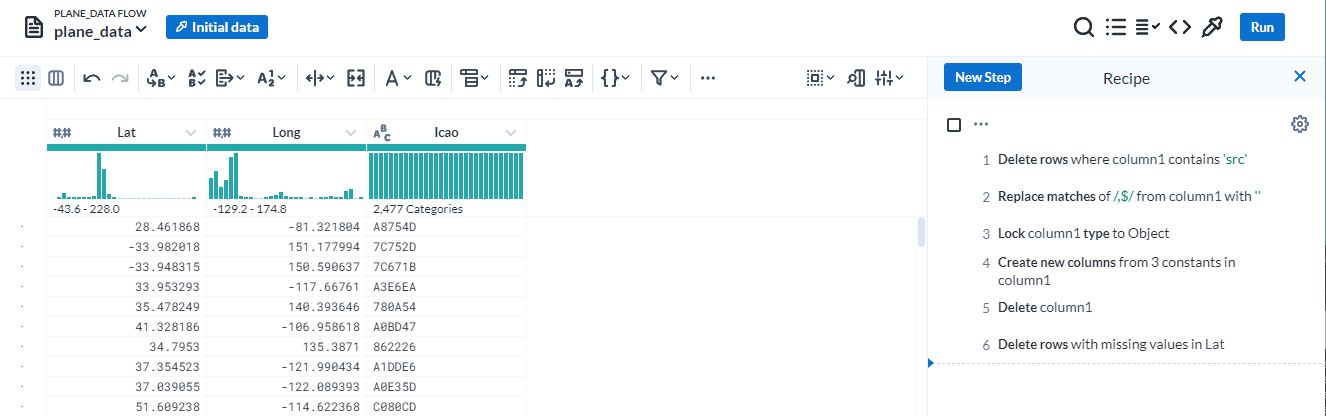
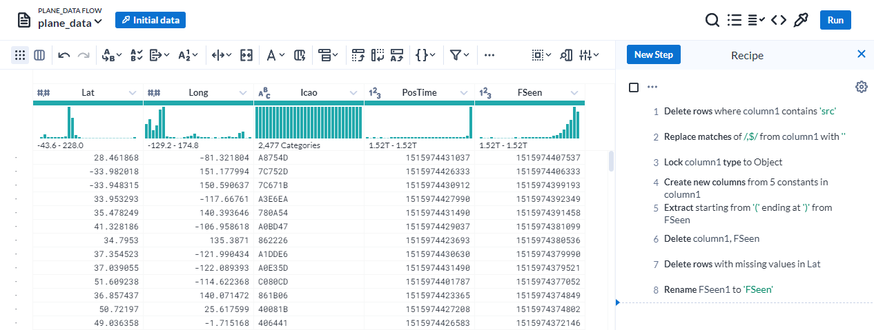
Once the JSON data was loaded into Google Cloud Dataprep, it was initially loaded as a single column with 7,432 rows. We needed to get this data into a format that was ready for analysis, specifically three columns that we are interested in: Lat, Long, and Icao. To do this, six steps were taken during the data cleaning:
- Delete rows where column1 contains “src”, which removed the first row.
- Replace matches of ,$ from column1 with nothing, which removes the comma located after each } on every row.
- Lock column1 type to an Object, which converts from string into JSON format.
- Create new columns from 3 constants in column1. This extracts the Lat, Long, and Icao columns from each row to create three new columns based on their corresponding values.
- Delete column1, since we no longer need the data from it.
- Delete rows with missing values in Lat, so that all values in the final data are not missing.
The below image shows that the JSON files were successfully loaded into Dataprep, and all the above steps were added to the recipe in order to create the new data:
After this, we then run the current job using the above data and load it into a BigQuery dataset to be used in the exploration. Below shows that the job was successfully finished:

Data Analysis (BigQuery)
The question of interest for this dataset is how many unique airplanes, identified by their ICAO, were in the area defined by Lat 44.497222 $\pm$ 0.2 and Lon -123.289444 $\pm$ 0.2. This pertains to the rectangle around the Corvallis, OR airport. In order to answer this, we will use BigQuery along with the dataset created from the Dataprep job. Below is the query used to answer this question, along with the output from BigQuery:
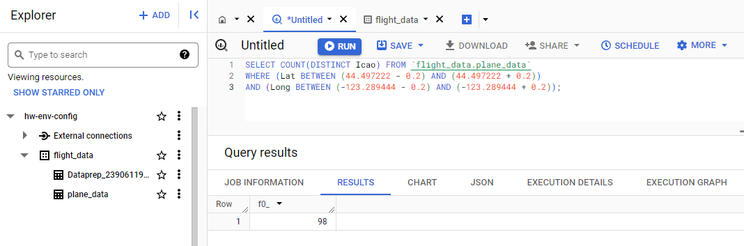
Looking at the provided output from BigQuery we can see that the data was successfully downloaded, transferred, scrubbed, and used in the analysis. There were 98 unique planes identified in our data which were in the Corvallis, OR airport.
PySpark & Dataproc
Data utilized in this project was a continuation of the previous work, but extended to utilize PySpark and Dataproc for running a much larger task. We aim to identify from the dataset the 10 airplanes which flew the farthest in a single day. However, there are known errors in the dataset in which the planes were recorded flying further than possible (i.e. faster and further than any plane is currently capable of by a substantial amount). In order to handle this, we must implement methods using PySpark in order to filter out bad data before running out Dataproc job. The below screenshot is the Dataprep job utilized to format the data and submit the job into the GS Bucket. Much of it is similar to previously discussed, but a few new steps were added:
Initial Job (PySpark & Dataproc)
For comparison, below is the screenshot of the Dataproc job output for the initial script that did not do any filtering. I had initially run this to ensure that everything was properly working. I also wanted to include it just to compare how the results differed, which seems to be by a large amount for both the top 10 planes and total distance flown on that day.
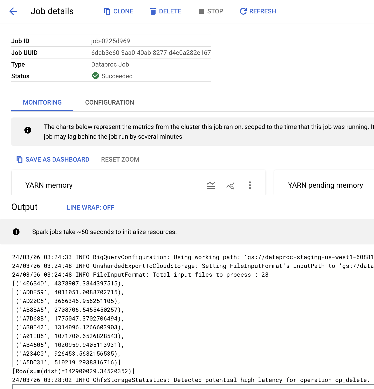
While looking around I found that the longest a commercial plane can fly in a day is estimate to be anywhere between 14,000 - 17,000 km depending on the number of stops and plane type. These numbers are vastly different than what we expected, and need to be filtered out using some type of method to handle outliers.
Filtering Outliers (PySpark)
Latitude & Longitude: The first step in filtering bad data was to exclude any observations with latitude and longitude values outside of the acceptable bounds. For latitude this ranges between [-90, 90] and for longitude this ranges between [-180, 180]. Most values seemed to fall in this range, but to ensure that it was correct they were filtered out right after the creation of the data frame. The below code handles this:
# ----- ADDED CODE FOR FILTERING LATITUDE (-90, 90) AND LONGITUDE (-180, 180) -----
## Most values are in appropriate ranges, but some seem to be outside of the valid values
## This will filter out any lat/long that are not plausible (reduce number of planes to
## calculate distance on, if any invalid readings are present).
df1 = df1.filter((df1['Lat'] >= -90) & (df1['Lat'] <= 90) &
                 (df1['Long'] >= -180) & (df1['Long'] <= 180))
IQR Method for Removing Outliers: The second step, after calculating all of the distances, was to filter outliers based on an IQR Method. Essentially this method takes the 1st and 3rd quartiles, takes the difference between them to find the interquartile range (range for middle 50% of the data), then subtracts 1.5IQR and adds IQR1.5 from the 1st and 3rd quartiles (respectively). This method aims to estimate the theoretical max/min based on these values, removing outliers. This is similar to a boxplot, whose bars represent these theoretical max/min. I slightly modified this to use the quantile values 0.2 and 0.8, instead of 0.25 and 0.75 for filtering the data, giving a slightly wider range of values to keep. Below is the code that implements this:
# ----- ADDED CODE FOR FILTERING DISTANCE BASED ON LOGICAL VALUES -----
## This is a slightly modified verision of using the IQR Method to filter values
## that are above what we would expect the min/max to be for distance. Usually it uses
## the 1st and 3rd quartiles, but I gave it slightly wider ranges in an attempt to not
## cut off possibly valid distances.
qu = df1.select(expr('percentile_approx(dist, 0.8)')).first()[0] # upper quantile
ql = df1.select(expr('percentile_approx(dist, 0.2)')).first()[0] # lower quantile
iqr = qu - ql # inter quartile range between qu and ql
iq_max = qu + abs(1.5*iqr) # find theoretical max (remove outliers)
iq_min = ql - abs(1.5*iqr) # find theoretical min (remove outliers)

# filter to only keep distance values in iqr method range
df1 = df1.filter((df1['dist'] <= iq_max) & (df1['dist'] >= iq_min))
Resubmitted Job (Dataproc)
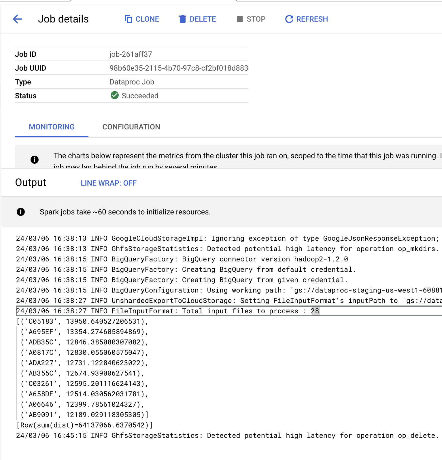
Below is the outputted values for the 10 planes that flew the farthest distance for the day, as well as the total distance flown by all planes. The values seem more reasonable, as looking around I found that the longest a commercial plane can fly in a day is estimate to be anywhere between 14,000 - 17,000 km depending on the number of stops and plane type. Compared to the initial results, the distances seem to be much closer to this expected range, so the filtering seems to work as intended. I believe the quantiles could be slightly expanded to include more data without catching too many extreme values, but that is something I’d have to play around with. The output for the job is provided below:
Both projects provided great insight on how to work with GC tools from obtaining data, cleaning/storing it, and running data analysis on both BigQuery and Dataproc. These tools will help me implement my own projects in the future, as well as transfer over to real world skills that will be used throughout my career.