Note: formatting is a bit strange since math equations cannot be written in the website files, and figure captions are not aligned. The following link provides the pdf in Google Drive for reading as well: Original Paper Link.
GitHub repository with the developed methods & code: GitHub Repo Link.
Abstract
Temperature data is inherently error prone, with reliance on the accuracy of the sensors and continuous readings that fall within expected ranges. The Decision Aid System (DAS) is an online tool for pesticide management and recommendation that relies heavily on these temperature readings for horticulture models in order to correctly identify and provide diagnosis. It is essential that quality control is applied to these temperature readings to ensure that the real time recommendations by these models correctly reflect the current environment being read by these weather stations. In this paper, we develop and evaluate approaches to estimating the parameters of a quality control system based on historical data of a weather station. Through cross-validation, stations are evaluated on varying years of input data in order to determine the necessary amount of historical data to successfully integrate a new station into the system. Our results suggest that each parameter varies for the necessary amount of prior data to effectively apply quality control on future data, but never exceeds 5 years.
Introduction
Quality control (QC) is an essential step in the data management process, ensuring that the data being collected meets a required standard for the given system it is utilized within. The Decision Aid System (DAS) incorporates historic weather data from a variety of sources including the WSU-AgWeatherNet, Weather Source, and Daymet in their forecasting models. The system relies on time-sensitive weather readings used in a variety of horticulture models that generate pest management recommendations for tree fruit farmers, and the accuracy of these readings directly corresponds to the success of these recommendations. Since temperature data is inherently error prone, QC becomes an essential step to ensure that the data being recorded and inputted into these models falls within expected ranges. As discussed by Celik et al. it is common to see fluctuations between high and low temperatures, but only within certain time frames. Considering the location at which the station is at, along with the time frame during the year in which the temperature occurs, a valid data reading in one month may be identified as an anomaly in another [1].
The aim of this project is to discover methods that can be applied to weather data readings across a variety of stations throughout the Pacific Northwest (PNW) in order to create a QC pipeline. We focus solely on temperature readings within this projects context, with two main components of interest: overall temperature ranges and differences between consecutive temperature readings. By discovering parameters to bound the overall temperature readings at a daily level, along with the parameters required to bound the allowed change in temperature at the monthly level, we have implemented a QC process that can be automated and applied to any station within the DAS database. Historic weather data from a variety of stations across the PNW collected by the DAS database between the years 2014 to 2023 is utilized for the project, with synthetic data being generated using the Daymet recordings [6] for validation across each station.
Background
Applying quality control (QC) to data encapsulates a large variety of methods ranging from ensuring data is complete and continuous by imputing missing values, to detecting outliers and correcting errors. Since this project works mainly on detecting outliers, we focus our discussion mainly on this area and provide background information on the types of errors that commonly occur along with the types of QC that can be applied to them. Summarized from Steinacker et al. on their work for data quality control [5], there are three main errors we see occur within temperature data: random, systematic, and gross errors. When discussing random and systematic errors, these commonly occur as a result of the instruments being utilized in recording the weather data. Since these readings are only an approximation, and equipment can be improperly calibrated or experience sensor drift, these slight variations are considered small scale errors. Although they are important to catch, they do not significantly impact the performance of a system as much as gross errors.
Gross errors define values that are rare in occurrence and large in magnitude, not following the distribution of the data. Commonly referred to as outliers, these values can have a high impact on forecasting in models and occur as a result of malfunctioning devices during data transmission [5. Pulling an example discovered during the project when exploring data on June 12, 2018 for station 115, temperature readings were steadily increasing from 40 to 60 degrees when data readings cut off and were marked missing. A random spike down to -20 degrees was recorded, and moments later the reading was back to 60 degrees. A combination of all three errors types, a sensor being replaced without the data transmission being turned off led to a reading far outside of the expected range. These types of errors are common within the DAS database, and need to be flagged for removal in a QC check before being inputted into any horticulture models.
The simplest and most extensively used algorithm of the automated QC checks is referred to as the range limit check, where measurements are compared against pre-defined upper and lower limits [7]. Measurements are flagged as valid or invalid based on the readings falling within or outside of these expected ranges, respectively. These calculated limits are station dependant and a soft limit is implemented when the ranges are required to vary according to their geographic areas, as well based on the time frame during the year when the data is recorded. In this project we implement two methods that allow for the soft limit to be found for any given station in the DAS database, which can then be applied in the automated QC pipeline.
Technical Approach and Methods
This section describes the methodology behind the implemented quality control (QC) checks, and to clearly define the problem, there are two main components that comprise the pipeline. The temperature bounds are the allowed minimum and maximum temperatures for a given time period, with a threshold applied to allow for slight variation in data readings. The delta bounds are the allowed minimum and maximum temperature changes between two consecutive readings, with a threshold applied to allow for slight variation. All temperatures are measured in Fahrenheit and come from the Decision Aid System (DAS) database, where readings are 15-minute intervals collected from weather station sensors across the PNW. For validating the methods, an algorithm was implemented in order to generate a synthetic dataset for each station using 2023 temperature data readings.
Overall Temperature Bounds
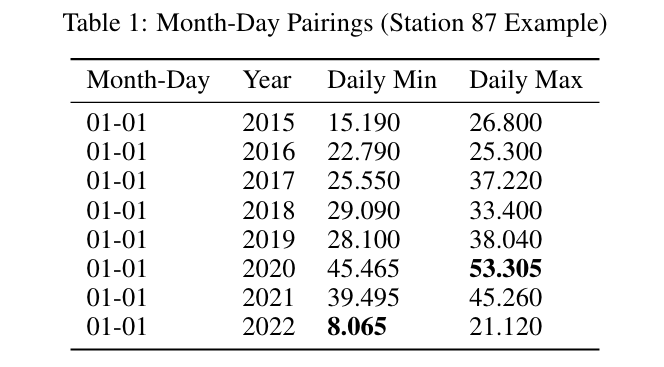
The first component of the QC system is to estimate the parameters utilized for bounding the overall temperature, ensuring that values fall within expected ranges for any given station. Through an initial visual exploration the number of bounds were tested at different levels of a yearly (1), seasonal (4), monthly (12), and daily (365) range. The data appeared to contain too large of a variation in temperature values, and as a result the daily estimate level was selected in order to capture these readings. To group data across all years and generate the bounds, month-day pairings are created by extracting the date from each temperature readings timestamp. From these pairings, each year in the stations data contains its own temperature readings for that given day from which the minimum and maximum are extracted. To account for outliers and missing values, the theoretical daily minimum and maximum are calculated by using the 0.01-quantile and 0.99-quantile, respectively. As represented in Table 1, once all values are produced, we then generate the estimated parameters for that day by grouping based on month-day pairings and extracting the minimum and maximum from their respective columns. This process is applied to all days across the dataset in order to create 365 daily bounds parameters, with the leap year date (2-29) being a duplicate of the previous days parameters (2-28). To allow for a slight window of error, a threshold of 15 degrees is added on top of the maximum and subtracted from the minimum to produce the initial daily estimates.
As a form of quality assurance to verify that no erroneous readings are calculated as bounding values, we apply a check using the monthly minimum and maximum estimated temperatures. To find these theoretical values, the interquartile range (IQR) method for detecting outliers [3] is applied such that $monthly_{max} = Q_3 + |1.5 * IQR|$ and $monthly_{min} = Q_1 - |1.5 * IQR|$, where $IQR = Q_3 - Q_1$. Similarly, a threshold of 15 degrees is applied to both the minimum and maximum estimates. Once these bounds are found for each month, we then replace any values within the daily minimum with the $max(daily_{min},, monthly_{min})$ and the daily maximum with the $min(daily_{max},, monthly_{max})$. Since we find the theoretical single value for the monthly minimum and maximum, any value outside of this range are interpreted as outliers and replaced. This process does not widen the bounds, but narrows them if the monthly estimates are lower or higher than their respective daily estimates.
In the final step, the bounds are smoothed to create a linear least squares line through the estimated data points using a Savitzky-Golay filter [4]. A window size of 15 and second order polynomial are used to fit the final line, creating 366 smoothed estimates for both the upper and lower daily temperature bounds. Refer to Figure 2 in Results section for visual representation of the smoothed bounding temperature estimates generated from the above process.
Delta Bounds
The second component of the QC system is bounding the difference between consecutive temperature readings, referred to as delta values. Similar to the temperature bounds, different levels of parameter estimation were explored and monthly (12) bounds were selected. Advanced outlier detection techniques were applied, but no success was found since the data is one-dimensional with a high frequency of values around 0 and normally distributed. As a result of this, a simple but robust technique for filtering outliers was required and the proposed of algorithm for detecting outliers using interquartile range techniques [3] was implemented. We slightly modified the bounds, where the 0.25-quantile (Q1) and 0.75-quantile (Q3) were replaced with the 0.1-quantile and 0.9-quantile, respectively. This allowed for slightly wider bounds in our estimation, since we saw an increasing number of valid readings in the tails of the delta distribution being incorrectly flagged. Algorithm 1 provides the implementation details for estimating the monthly delta minimum and maximum bounds, with the threshold being set to 1 degree to allow for slight variation in sensor readings.
Algorithm 1: Algorithm for estimating monthly delta bounds.
Data: 2D array of temperature readings (N_DAYS x 96)
Result: 2D array of per month min/max delta estimates (12 x 3)
x ← 1D array of flattened 2D input data
d ← all values of x[cur] - x[prev], where prev = cur − 1 and 1 ≤ cur ≤ len(x)
d ← 0 inserted in first position (account for first day)
v ← d reshaped as original 2D input data shape, (N_DAYS x 96)
iqr_est ← empty dataframe to hold estimates, columns: [month, lower bound, upper bound]
for m ∈ {1, 2, . . . , 11, 12} do
  s ← v subset for the current month, m, across all years in data
  qu ← quantile(s, 0.9)
  ql ← quantile(s, 0.1)
  iqr ← qu − ql
  iq_max ← qu + |1.5 ∗ iqr| + threshold
  iq_min ← ql − |1.5 ∗ iqr| − threshold
  iqr_est ← new row with values [m, iq_min, iq_max]
end
return iqr_es
Synthetic Data Generation
The weather readings in the DAS database contain unknown errors in both minimum/maximum temperature and delta values, but cannot be labelled manually due to the number of data points represented in each station. In order to accurately validate the parameters that are generated from the above methods, a synthetic dataset of 15 minute temperature readings for the 2023 year must be created for each station. In order to implement this, we provide the latitude and longitude for a given station to query the daily minimum and maximum temperature readings from the Daymet API [6] across 2023. Daymet provides historic data for long-term weather variables through statistical modeling techniques, and is a product of the Environmental Science Division at Oak Ridge National Laboratory along with the supported of NASA and the U.S. Department of Energy. For this reason, we make the assumption that the data provided is reliable with no errors present, and fall within expected ranges for any given location. The queried values are only daily minimum and maximum temperature readings, and must be converted into 15 minute intervals to match the provided format from DAS.
As discussed by Chow et al. [2] in their paper for generating hourly temperature values using daily maximum, minimum, and average values, we implement their algorithm in order to create hourly readings and link these values across an entire year. By knowing the next temperature ($T_{next}$) and previous temperature ($T_{prev}$), along with the times at which they occur ($t_{next}$ and $t_{prev}$ respectively), we can generate hourly temperature readings using the following algorithm: $$ T(t) = \left( \frac{T_{next} + T_{prev}}{2} \right) - \left( \frac{T_{next} - T_{prev}}{2} \right) \times cos \left( \frac{\pi(t - t_{prev})}{(t_{next} - t_{prev})} \right) $$
Note that T_next and T_prev both take on the values of minimum and maximum temperature dependent on what time of day we are linking together. For our synthetic data we use the Sin (14R-1) method, where the time at which the maximum temperature occurs is assumed to be the hour 14 for any given day. As provide in the paper, we take the average time at which the minimum temperature is recorded and assume it always occurs at hour 5. Through this algorithm, we generate 24 readings per day across the year 2023 using the Daymet temperature readings. We then use cubic interpolation, along with random noise between -1.8 and +1.8 degrees, to generate the 15 minute intervals between these hourly readings. Provided in Figure 1, the temperature for a single day provided by DAS and produced through the above method are compared to visualize the similarity for a single station. Data produced by only using interpolation, without the above algorithm, is also provided for reference. Note that the above method for creating the data is wrapped in a function, which can take any station in DAS to extract the necessary information and produce an entire year of synthetic temperature readings that will be utilized in the results section of the paper.
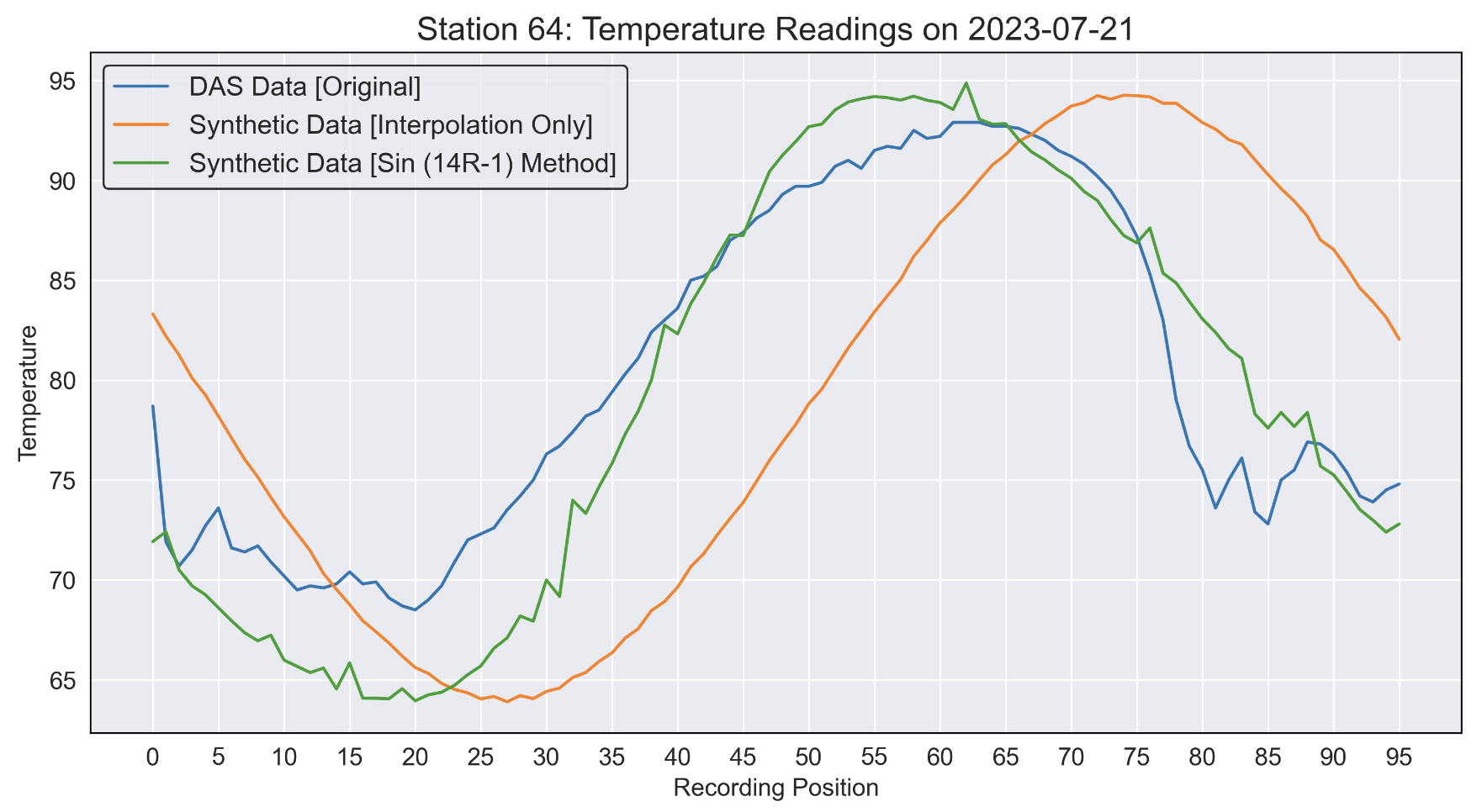 Figure 1: Synthetic vs DAS data (Station 64 single day example).
Results
To evaluate the effectiveness of the generated parameters for the QC system, a modified version of k-fold cross-validation is applied to 18 stations across the state of Washington in a variety of different environments. All stations contains 8+ years of historic data such that the cross-validation can be performed equivalently for each. The end goal is to answer the question: how many years of data is necessary in order to accurately estimate these parameters for any given station in the DAS system, such that they can be integrated into the QC pipeline? To do this, we perform the modified k-fold cross-validation by varying the number of years used for estimating the parameters, ranging from 1 to 8 years. For each set of years, 5 different folds are chosen at random from the provided years of available data in order to estimate the parameters. For instance when utilizing 3 years of historic data to estimate parameters, 5 different random but reproducible combinations of the years 2014 - 2022 are selected and subsetted from the DAS temperature readings. This process is repeated for each number of estimation years, and the average F1 score of each parameter is recorded in order to obtain the results.
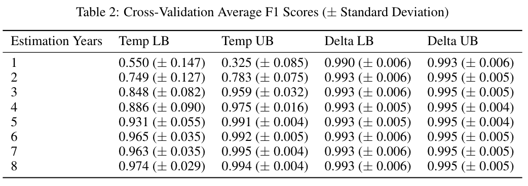
As discussed in the previous section, each station will be validated on their own unique synthetic data set with randomly injected errors. Since the synthetic data is assumed to be fully correct, random errors are injected into the data and labels are produced so that they may be evaluated based on an F1 score. For the provided results, 250 random spikes in the temperature were inserted of either $\pm$50 degrees to verify the daily minimum and maximum temperature parameters. Similarly, 250 random spikes in the temperature were inserted of either $\pm$10 degrees in order to verify the monthly delta parameters. All randomly injected errors are marked as incorrect readings in the validation labels, with all other data points being set as valid temperature readings. Once results were acquired for each of the 18 stations, they were then averaged and the standard deviation was recorded for each parameter, which is presented in Table 2.
Overall Temperature Bounds
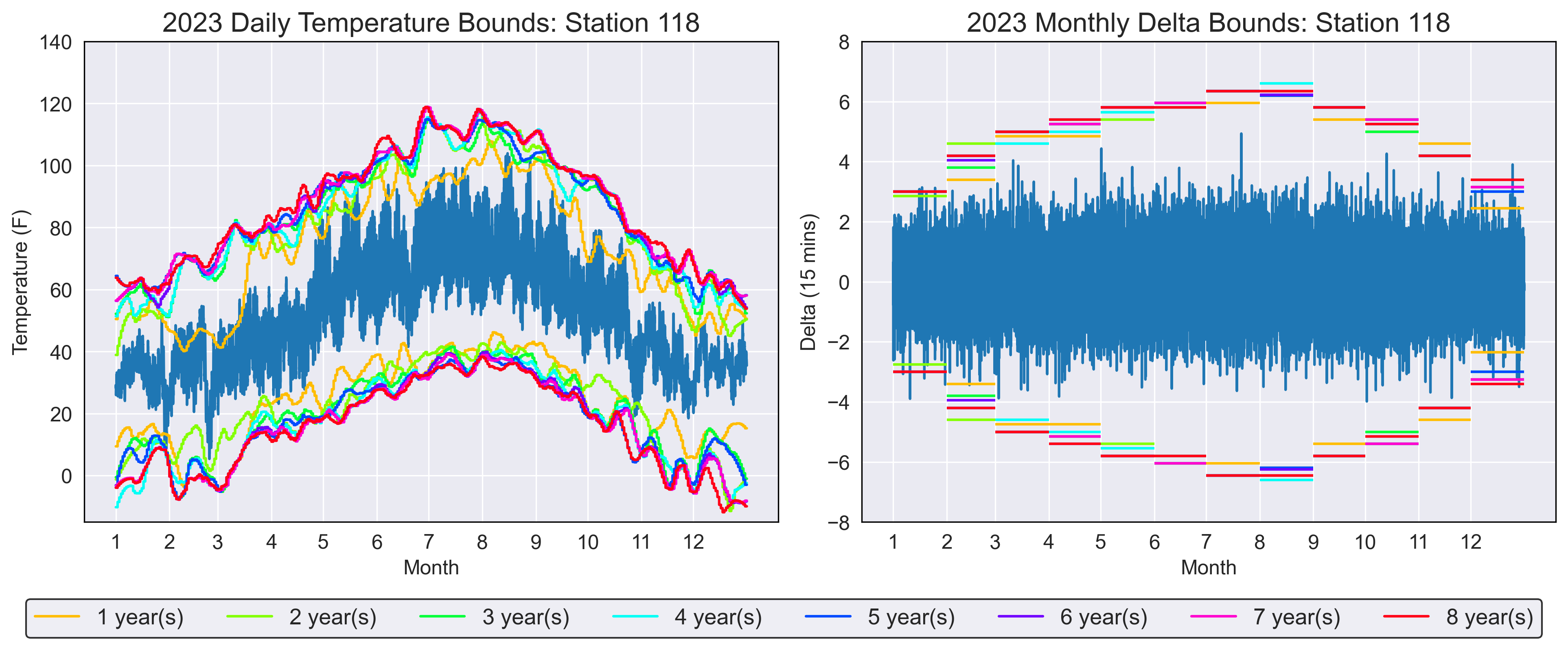 Figure 2: Parameters produced from varying estimation years, plotted on 2023 synthetic temperature data (Station 118 example).
Estimating the lower bound for the daily temperature parameters has proven to be less accurate than expected, requiring much higher amounts of data than previously anticipated. From results presented in Table 2, we see the average F1 score begins low and continues to increase as more readings are incorporated into the estimation data. We also see a high variance in the average F1 score for under 2 years of estimation data, ranging between 0.3 and 0.8 depending on the station. This provides the insight that not all stations require the same number of estimation years, with some being sufficiently accurate with 2 years of data and others under performing with 8 years. Although, on average, 5 years is sufficient for an accurate daily lower bound parameter, the average F1 score continues to increase as more data is incorporated in the estimation. Based on the per-station breakdown of the average F1 score in Figure 3, we see a variety of stations whose F1 score has either plateaued or are continuing to approach 1.0 as the estimation years increase. All stations are moving towards convergence of fully accurate lower bounds and as more readings are incorporated into the estimation data, we would expect these parameters to be reached.
In contrast, estimating the upper bound for the daily temperature parameters has proven to be straightforward and follow the same general pattern. From results presented in Table 2, although the average F1 scores is initially significantly worse than the lower bound, it quickly converges and becomes accurate with only 3 years of estimation data. We see very low variance in this parameter, which is confirmed by the per station F1 results is Figure 3. All stations converge at nearly the same point, plateauing around 5 years of estimation data and achieving an average F1 score of approximately 0.99. Contrary to the lower bound insights, the upper bound is universal in the amount of data required to estimate accurate parameters and does not depend on the station.
Bounds are estimated such that they capture all valid temperature readings within the estimation data time frame, and as a result of yearly temperature variation we typically see the bounds expand. As new daily minimum and maximum’s are discovered through the inclusion of more data, bounds are adjusted to decrease and increase, respectively. Although it is of high importance to include the previous year in estimating the current years parameters, it is not sufficient to only use a single year worth of readings. As previously discussed, the amount of data required for estimating these parameters is not universal and is highly dependant on the station. However we can conclude that, on average, 5+ years of historic data is required in order to obtain accurate estimations for the daily temperature bounds and integrate a new weather station into the QC pipeline. Based on results in Table 2, although 5 years is sufficient, accuracy only increases as more data is utilized for these parameters and including all available recordings is the recommended approach.
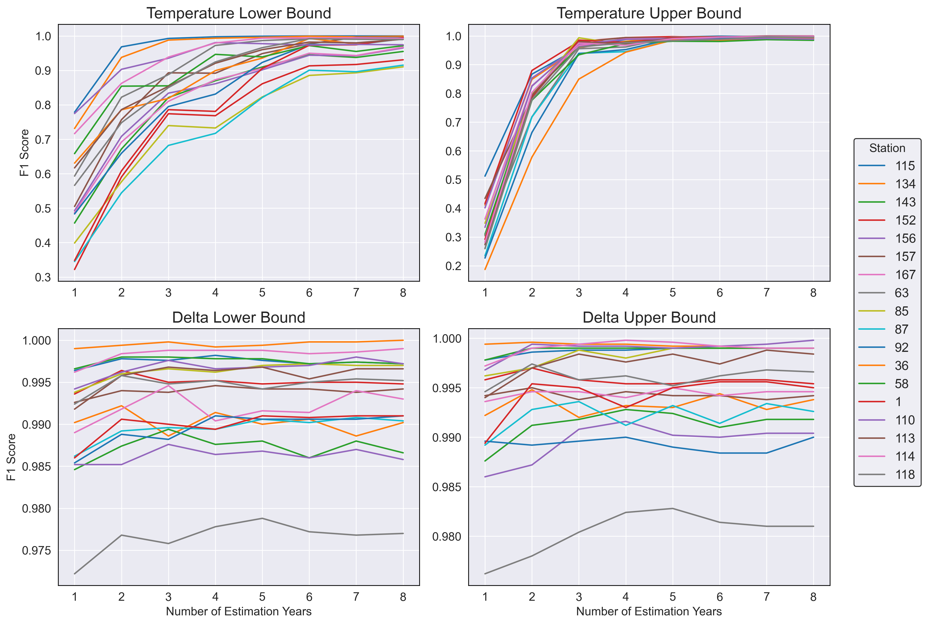 Figure 3: F1 scores for cross-validated stations, across each number of years used for estimating parameters.
Delta Bounds
Temperatures can vary from year to year, but the difference between consecutive 15-minute readings has been found to be consistent across each. Despite the number of years used in estimating the parameters, the average F1 score presented in Table 2 remains constant after 2+ years of estimation data. Although we do see the general pattern in Figure 2 of narrower bounds during winter months, and expanding bounds during summer months, these bounds concentrate around similar values in each month for any number of estimation years. Since the majority of the data is centered around zero, and is approximately normally distributed for each month, the implemented methods produces nearly symmetrical bounds around this central value. Estimates for the monthly upper and lower bound are unique for each station, but follow the same general pattern of symmetry around the central value of zero.
Although a great amount of insight is not found from the results on the delta estimation, Figure 3 does provide a breakdown of the per-station F1 score across all estimation years. Although we see a very small amount of variation, the number of estimation years does not have a significant effect. Based on this, we conclude that only a single year of historic data is necessary in order to obtain accurate estimations of the monthly delta bounds and integrate a new weather station into the QC pipeline. Including more than a single year will not negatively impact the accuracy of the parameters, but is not necessary based on the provided results.
Advice for Future Students
Although there were many learning experiences that were discovered throughout the duration of the project, there are two main pieces of advice I would suggest. The first is to simplify the problem before moving to more complicated techniques. Implementing complex models was my first thought for estimating the bounds, looking at the data as a time series problem using some type of LSTM model capable of predicting temperature values from which the minimum and maximum bounds could be extracted from. However, through extensive data analysis, it became apparent that weather patterns were common across years and a general pattern could be extracted using statistical techniques rather than advanced machine learning concepts.
The second piece of advice I would suggest is to have a clear problem definition with an end goal, and to be sure you fully understand the problem before beginning. I spent longer than necessary thinking I understood the problem but working towards a different end goal than what was expected. Sitting down with the project partner’s and advisor to discuss and write down a clear problem definition with requirements made the project much more clear, and had I taken the initiative to do this in the beginning, would have allowed more time for working on the final product.
Looking forward on what can be expanded upon from this project, we focused mainly on a single reading from weather sensors (temperature). However there are a variety of variables such as elevation, latitude, longitude, and other attributes that could also be utilized to potentially create more accurate parameters. Similarly, neighboring stations will have similar temperature readings and clustering them together based on location to implement further quality checks on parameters is another area of interest that is being discussed. Finally, there are other readings from these sensors which require quality control to be applied such as humidity, precipitation, soil temperature, etc. Although similar methods can be applied, they may require slight modifications based on the distributions which the data follows. Expanding the current methods to all readings that are utilized by the DAS models will allow us to ensure the most accurate recommendations are being made.
References
[1] Mete Celik, Filiz Dadaser-Celik, and Ahmet Dokuz. Anomaly detection in temperature data using dbscan algorithm. 06 2011.
[2] D.H.C. Chow and G. Levermore. New algorithm for generating hourly temperature values using daily maximum, minimum and average values from climate models. Building Services Engineering Research Technology - BUILD SERV ENG RES TECHNOL, 28:237–248, 08 2007.
[3] Vinutha H P, B. Poornima, and B. Sagar. Detection of Outliers Using Interquartile Range Technique from Intrusion Dataset, pages 511–518. 01 2018.
[4] Abraham. Savitzky and M. J. E. Golay. Smoothing and differentiation of data by simplified least squares procedures. Analytical Chemistry, 36(8):1627–1639, 1964.
[5] Reinhold Steinacker, Dieter Mayer, and Andrea Steiner. Data quality control based on self- consistency. Monthly Weather Review, 139:3974–3991, 12 2011.
[6] P.E. THORNTON, M.M. THORNTON, B.W. MAYER, N. WILHELMI, Y. WEI, R. DE- VARAKONDA, and R.B. COOK. Daymet: Daily surface weather data on a 1-km grid for north america, version 2, 2014.
[7] Igor Zahumensky. Guidelines on quality control procedures for data from automatic weather stations. 01 2004.